
Climate change is altering the frequency and severity of extreme weather events such as wildfires, floods and windstorms. Over the last few years, it has become increasingly common for insurers to adjust catastrophe model output to reflect these changes, driven in part by new regulatory requirements.
While most of the focus has been placed on methods for adjusting frequency-severity relationships, little attention has been given to scenario completeness, particularly in the tail of the distribution, where some of the most severe impacts are expected to materialize. As a result, insurers could be underestimating the physical risks to which they are exposed.
See also: How AI Can Help Insurers on Climate
The dominance of short return periods
When it comes to physical climate change impacts on the insurance industry, one of the most cited research papers is Knutson et al. (2020), which presented a synthesis of the expected changes in global tropical cyclone activity for a 2°C warming scenario. Many insurers have used this paper as a basis for adjusting the frequency and severity of tropical cyclones in catastrophe models to quantify the effects climate change could have on insurance claims.
But if you have ever applied the Knutson et al. frequency-severity adjustments to a catastrophe model, you might have noticed something that at first seems counterintuitive: After the correction, short return period losses tend to increase more percentage-wise than those in the tail of the distribution. Figure 1 shows the impact of a 20% increase in the number of Category 4 and 5 landfalling hurricanes in a U.S. tropical cyclone model. The largest effect is seen near the bottom of the exceedance probability (EP) curve, with a 15% increase at the one-in-two-year return period loss. In comparison, tail losses around the one-in-200-year return period only increase by 5.5%.
The reason for this inconsistency is simple: Short return periods compose most of the loss distribution, so adding in events fattens this portion of the EP curve the most. In a 100,000-year simulation, for example, 90% of the years are at or below the one-in-10 return period. This means that if a new event is included at random, it has a 90% chance of being added to a year at or below the one-in-10.
This effect is counterintuitive because we know that the upper tail of the distribution is likely to contain some of the most severe physical consequences of climate change, particularly under higher emission pathways. Does it, therefore, stand to reason that the percentage increase in tail return periods should be lower compared with shorter return periods? What could we be missing from our scenarios that explains this?
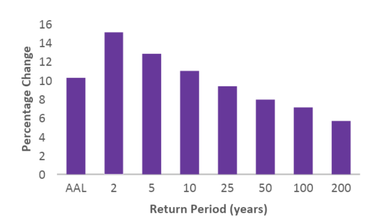
Figure 1: The percentage change in losses for a 20% increase in the number of Category 4 and 5 landfalling hurricanes in a U.S. tropical cyclone model
Unquantified tail risks
As Nassim Taleb has written in relation to financial markets, traditional models do not handle fat-tailed events well. This limitation means that important things are likely to be missing from the view of risk. The same is true for traditional catastrophe models when it comes to climate change: While frequency-severity distributions can be conditioned for various climate states, they underestimate the true tail risk, especially when we start to think about things like tipping points, feedback loops and systemic risks.
This is not to diminish the usefulness of catastrophe models. They combine detailed hazard modeling, engineering knowledge and information on exposures in ways that other tools, such as climate models, cannot. However, just as insurers evaluate and quantify non-modeled risks today, for example under Solvency II, they need to deploy the same thinking and methodologies when it comes to climate change adjustments and scenarios.
For example, traditional risk assessment methods often focus on a single hazard at a time, but research indicates that the likelihood of hazards co-occurring – such as extreme winds and precipitation – will increase in a warmer world. An increase in cross-peril correlation will lead to increased tail risks, but most insurers are not currently considering this possibility in their modeling.
There is also mounting evidence that some tipping points, such as the collapse of ice sheets or the melting of permafrost, may be triggered at a global mean temperature of 1.5°C. Such events would have far-reaching ramifications, with severe consequences not just for the insurance industry but society as a whole. The world is expected to reach 1.5°C at some point in the 2030s, meaning some of these fat tail outcomes could be closer than many realize.
In addition to these direct physical risks, there are also several indirect effects that are frequently overlooked, including supply chain disruption, food insecurity, geopolitical conflict and infrastructure failure. All of these have the potential to manifest as systemic effects, which will stress global economies.
See also: Glimmers of Good News on Climate (Finally)
Climate Amplification Factors
The breadth and complexity of climate change tail risks mean that careful consideration is required when incorporating them into our modeling. In some situations, it will be possible to explicitly simulate the effects within existing frameworks – for example, cross-peril correlations can be included in simulation-based capital models. However, it will be more challenging for other risks, particularly those with socio-economic and systemic components.
Fortunately, there is an analogue in current catastrophe modeling frameworks when it comes to representing socio-economic factors that are difficult to quantify: post-event loss amplification (PLA). PLA is applied to the most severe events, such as Hurricane Katrina in 2005, to account for a range of complex tail sources of loss, including economic demand surge, long-term evacuation and systemic economic problems.
The same approach could be used to model climate change tail risk using “climate loss amplification” (CLA). The more severe an event, the larger the CLA factor, reflecting the increasing likelihood of socio-economic effects materializing, such as geopolitical conflict and infrastructure failure.
When you next think about building or updating your climate change scenarios, remember to consider not only how to best adjust frequencies and severities but also the completeness of your risk assessment.